GATE questions Gravity method

GATE 2009

1. Which of the following parameters is uniquely resolved by residual gravity anomaly data

(a) lateral density contrast 
(b) excess/deficit mass 
(c) absolute density 
(d) geometric dimensions of geophysical model

2. The presence of crustal root beneath a mountain chain can be best explained by 

(a) Pratt's model                         (b) Airy's model 
(c) Vening Meinesz model         (d) Plume model

3. For under water gravity measurements, the following correction is needed: 

(a) Prey correction         (b) Free-air correction 
(c) Bouguer correction   (d) Isostatic correction

Common Data for Questions 4 and 5: 

The peak gravity anomaly over a 2-D line mass of circular cross-section (horizontal cylinder) of density contrast 500 kg/m3 is 1.674 mGal. The anomaly decreases to 0.837 mGal at a distance of 500 m along a principal profile. The universal gravitation constant, \(G = 6.6667 \times 10^{-11}\ \  m^3sec^{-2}kg^{-1}\). 

4. The depth (m) to center of line mass and radius (m) of the horizontal cylinder are = 

(a) 500, 199.80 
(b) 200, 150.93 
(c) 200, 100.33 
(d) 100, 60.37 56. 

5. Hence compute the excess mass per unit length (kg/m) of the line mass 
(a) \(11.0 \times 10^{7}\),     (b)\(9.0 \times 10^{7}\)   
(c) \(6.27 \times 10^{7}\)     (d)\(3.67 \times 10^{7}\)

GATE 2010

1. If the average crustal thickness is 35 km and the height of a mountain is 5 km above mean sea level the crustal thickness based on Airy's model beneath the mountain will he approximately 
(a) 35 km     (b) 40 km     (c) 50 km     (d) 70 km

2. The equipotential sur face over which the gravitational field has equal value is known as
(a) geoid     (b) spheroid     (c) ellipsoid     (d) mean sea level

3. Among the following, the best reconnaissance method for determining basement configuration of sedimentary basins is 
(a) gravity method     (b) self potential method 
(c) seismic method     (d) electromagnetic method

4. The gravity value measured at the base of a 10 m tall building is 40 mGal. The value at the top of the bullding ignoring its mass is close to 
(a) 20 mGal     (b) 37 mGal     (c) 40 mGal     (d) 43 mGal

5. Upward continuation technique filters ________ wavelength anomalies and ____ their amplitudes. 
(a) short, reduces     (b) long, enhances     (c) long, reduces     (d) short, enhances

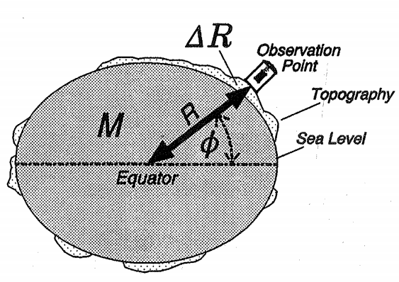
Common Data (or Questions) 

The terrain correction in gravity method accounts for topographic relief in the vicinity of the observation point. The Bouguer slab assumes the topography around the observation point to be flat. In the figure below, the Bouguer slab thickness is h and the hollow portion P lies within the Bouguer slab. Q and Rare parts of the topography
6. In the region P, the terrain correction is 
(a) half of that in R (b) negative (c) zero (d) positive 

7. In the region Q, the terrain correction is required to account for 
(a) hollow portion P 
(b) reduced gravity due to excess mass in portion Q 
(c) increased gravity due t o excess mass in portion Q 
(d) over-correction of Bouguer slab

GATE 2011

1. The acceleration due to gravity (g) and universal gravitational constant (G) are related by the expression (Me and Re are the mass and radius of the earth, respectively)


2. Gravity measurement is made on a ship sailing at the speed of 6 knots in the direction N65°E at 20°N latitude. The Eotvos correction (in mGal) is 
(a) +38.5 (b) +24.5 (c) – 35.5 (d) – 39.5

Statement for Linked Answer Questions

A gravity survey is conducted over a highly compact ore deposit (spherical shape). Bouguer anomaly values reduced along a profile are given below.


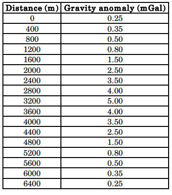
3. What is the depth to the center of the ore deposit? 
(a) 3100 m (b) 1820 m (c) 1560 m (d) 1450 m 

4. What is the excess mass (in metric tons) by the deposit? 
(a) 1.615 × 10^8 (b) 2.165 × 10^8 (c) 1.312 × 10^9 (d) 1.825 × 10^9

GATE 2012

1. Bouguer correction is applied to correct for the gravity anomaly due to mass between station location and 
(a) mean sea level     (b) local datum plane 
(c) base of upper crust     (d) Mohorovicic discontinuity

2. The change in gravity caused by Earth’s tides on the land surface in a complete tidal cycle is in the range of (in milligal) 
(a) 0.1 to 0.2 (b) 0.2 to 0.3 (c) 0.3 to 0.4 (d) 0.4to 0.5

GATE 2013

1. The acceleration due to gravity, 'g' is maximum at 
(a) equator (b) poles (c) mid-latitudes (d) sub-tropical regions

2. Which of the following is useful to estimate the depth to the centre of a spherical body from a gravity anomaly curve? 
(a) Surface integration (b) low-pass filtering Volume integration (c) Twice the absolute maximum (d) Half-width of the anomaly

3. If L, B, F and T respectively stand for Latitude correction, Bouguer correction, Free-air correction and Terrain correction, then the order in which they will have to be applied for gravity data analysis is 
(a) LFBT (b) LBTF (c) FLBT (d) TBLF

GATE 2014

1. The International Gravity Formula predicts the theoretical gravity value at a given point assuming a 
(a) non-rotating homogeneous spherical earth model 
(b) decreases rotating inhomogeneous spherical earth model 
(c) rotating homogeneous oblate spheroidal earth model 
(d) rotating inhomogeneous oblate spheroidal earth model

2. Compute the maximum value of gravity anomaly in µGal over a buried sphere from the following data: 
Radius of a sphere = 5 m 
Depth to centre of sphere =11 m 
Density contrast = 0.1 gm/cc 
G = 6.673 × 10– 8 dyne-cm2 /gm2 

(a) 2887.58 (b) 288.76 (c) 28.88 (d) 2.89

GATE 2015

1. The shape of the earth is best described as 
(a) spheroid (b) prolate ellipsoid (c) ellipsoid (d) oblate spheroid

2. Considering the Airy isostatic compensation for a mountain having elevation of 2.0 km above the mean sea level at a point P, the thickness of its root below P would be _________km. (consider densities of crustal rocks and upper mantle as 2.7 g/cc and 3.3 g/cc respectively).

3. . The Bouguer anomaly obtained after applying all necessary corrections is due to 
(a) topographic undulations above the datum 
(b) increase in densities of crustal rocks with depth 
(c) lateral density variations 
(d) vertical density contrast across Moho

GATE 2016

1. According to Airy’s model, gravity anomalies for fully isostatically compensated topography are characterized by 
(a) negative Bouguer anomaly and positive free-air anomaly. 
(b) positive Bouguer anomaly and negative free-air anomaly. 
(c) zero Bouguer anomaly and negative free-air anomaly. 
(d) positive Bouguer anomaly and zero free-air anomaly.

2. The value of free-air correction (assuming sea level as datum plane) at an elevation of 150 m is _________ mGal.

3. A spherical cavity of radius 8 m has its centre 15 m below the surface. If the cavity is full of sediments of density \(1.5 \times 10^3 kg/m3\) and is in a rock body of density \(2.4 \times 10^3 kg/m3\), the maximum value of its gravity anomaly is __________ mGal.

4. Match the items (listed in Group I) with the corresponding corrections applied for reduction of marine gravity data (listed in Group II). 


(a) P-4; Q-3; R-1; S-2 (b) P-2; Q-3; R-4; S-1 (c) P-4; Q-1; R-2; S-3 (d) P-3; Q-1; R-4; S-2

GATE 2017

1. The normal gravity formula (for e.g. GRS80) is a function of 
(a) geocentric latitude (b) geodetic latitude (c) longitude (d) altitude

2. Given the Bouguer density of 2.8 g/cc, the Bouguer correction for a gravity station at an elevation of 30 m above the datum is ____ mGals. (Use \(\pi\) = 3.14)

GATE 2018

1. The geoid can be best defined as 
(a) an oblate spheroid that best approximates the shape of the earth. 
(b) a surface over which the value of gravity is constant. 
(c) the physical surface of the earth. 
(d) an equipotential surface of gravity of the earth.

2. Which one of the following corrections is always added during reduction of the observed gravity data? 
(a) Latitude     (b) Free-air     (c) Bouguer     (d) Terrain

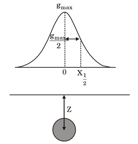
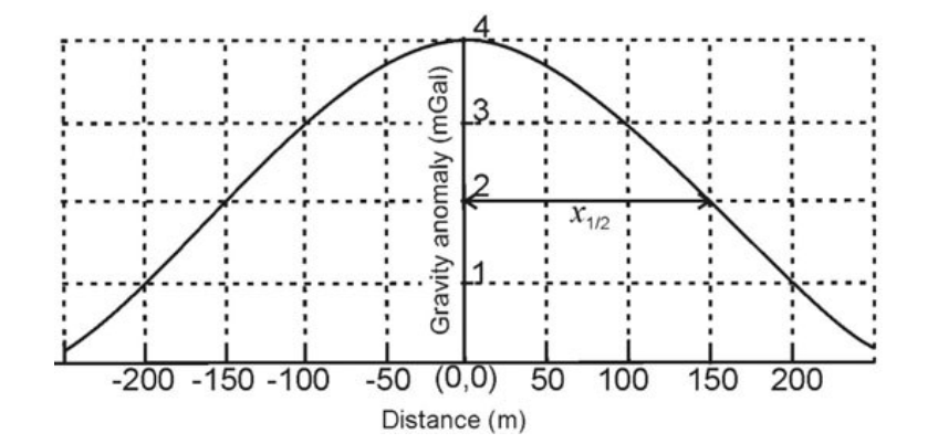
3. In the figure below, Z denotes the depth to the center of a buried sphere from the surface and \(X_{1/2}\) denotes the half-width of the profile at half the maximum value of gravity. Then, the ratio \(\frac{Z}{X_{1/2}}\) is ________.


4. Two survey vessels with shipborne gravimeters are cruising towards each other at a speed of 6 knots each along an east -west course. The difference in gravity readings of the two gravimeters is 63.5 mGal at the point at which the survey vessels cross each other. The latitude along which the survey vessels are cruising is ______ °N.

5. A gravity reading is taken in a stationary helicopter hovering 1 km above mean-sea level at a particular location. The difference in the value of g measured in the helicopter and at mean sea level vertically beneath the helicopter is ____________ mGals.

GATE 2019

1. Which one of the following is only a correction and not a reduction in the computation of gravity anomalies with respect to a datum? 
(a) Free air     (b) Bouguer     (c) Terrain     (d) Isostatic

2. Assuming Airy isostatic compensation, the depth to the Moho from a point located 2 km above the mean sea level is _____ km. (round off to 1 decimal place). (The depth of compensation T for the crust at mean sea level is 30 km, the density of crust and upper mantle are 2.67 gm/cc and 3.30 gm/cc, respectively).

3. In gravity anomalies, the ‘Indirect effect’ mainly arises from__________. 
(a) the sources outside the area of investigation 
(b) improper instrument drift 
(c) effect of mass lying between the geoid and ellipsoid 
(d) short-wavelength uncompensated masses in the subsurface

4. Which one of the following statements about the gravity anomalies on land is CORRECT? 
(a) Free-air and Bouguer anomalies are always positively correlated with elevation 
(b) Isostatic anomalies are not useful to understand the crustal heterogeneities 
(c) Vertical derivatives are used to enhance the gravity effects of deep-seated bodies 
(d) X-horizontal gradient \(dg/dx\) map enhances/sharpens anomalies of bodies trending N-S (X-East, Y-North, Z-downward).

5. In an abandoned mine-site, three hollow spherical cavities are located below the surface centered at depths of 50, 100 and 150 metres. Assuming that residual gravity is low due to each one of these cavities are small (~ 0.05 mGal), do not interfere and can be detected by the gravimeter, the most ideal (largest) grid spacing for carrying out the gravity surveys in order to correctly delineate these cavities is __________ metres, (round off to the nearest integer).

GATE 2020

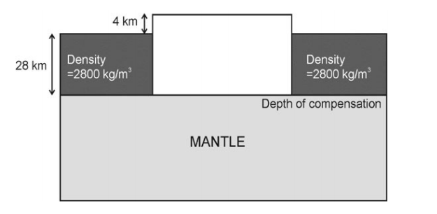
1. A 4 km-high plateau is isostatically compensated as shown in the figure. Assuming Pratt’s hypothesis of isostasy, the calculated density of the plateau is _____ kg/m3.

2. International gravity formula is based on which one of the following models? 
(a) Non-rotating homogeneous spherical Earth model 
(b) Non-rotating homogeneous oblate spheroidal Earth model 
(c) Rotating homogeneous oblate spheroidal Earth model 
(d) Rotating inhomogeneous spherical Earth model

3. A micro-gravity survey with appropriate station spacing is performed to detect a subsurface spherical cavity in a bedrock of density 2500 kg/m3. The depth to the center of the cavity is 4 m from the surface and the elevation measurement accuracy of the surveying instrument is 0.1 m. The smallest cavity that can be detected by the survey must have a radius greater than _______ m. (Round off to 1 decimal place) (Assume \(G = 6.673 \times 10^{-11} m^3kg^{–1}s^{–2}\)).

4. The gravity anomaly over a spherical ore body is shown in the figure below. The calculated excess mass due to the ore body will be _______ × 1010 kg. (Round off to 1 decimal place) (Assume \(z = 1.3 \times x_{1/2}\); \(G = 6.673 \times 10^{-11} m^3kg^{–1}s^{–2}\)).


Share:

Corrections for gravity data


Free Air Gravity Anomaly 

Gravity observed at a specific location on Earth's surface can be viewed as a function of three main components:

  1. the latitude (\(\phi\))of the observation point, accounted for by the theoretical gravity formula; 
  2. the elevation (\(\Delta R\)) of the station, which changes the radius (R) from the observation point to the center of the Earth; and 
  3. the mass distribution (M) in the subsurface, relative to the observation point.

Indirect effect and Cogeoid

When removing the effect of the Bouguer plate and/or the train undulations, we actually disregard the masses above the geoid. In other words, when using the Bouguer anomaly, we mathematically change the real distribution of masses, the potential of the earth and hence even the geoid. This distortion is usually called the indirect effect of mass removal and the surface thus distorted is known as Compensated Geoid or Cogeoid.

Geophysical indirect effect

The indirect reduction or correction, which is applicable to the calculation of all gravity anomalies, is the gravitational effect resulting from the use of different vertical datums for establishing the height and theoretical gravity at a station’s position. It represents the difference between the geoidally obtained gravity measurements and the ellipsoidally referenced mapping system.

The indirect effect combines the gravitational effect of the difference in height between the geoid and ellipsoid at the station and the mass effect of the included material.

Assuming a horizontal layer of thickness equal to the difference in height (the geoidal height or undulation) and a density of 2,670 kg/m3, the effect is $$g_{ind} = (0.3806 − 0.1119)N = 0.1976 \ N $$ where N is the geoidal height in meters and \(g_{ind}\) is the indirect reduction in milligals. 

If the geoid is above the ellipsoid, the indirect reduction has the same sign as the elevation correction and vice versa.


Share:

Filter

Share:

Sampling theorem

A continuous-time (or analog) signal can be stored in a digital computer, in the form of equidistant discrete points or samples. The higher the sampling rate (or sampling frequency, \(f_S\)), the more accurate would be the stored information and the signal reconstruction from its samples. However, high sampling rate produces a large volume of data to be stored and makes necessary the use of a very fast analog-to-digital converter.

If the continuous signal observed between \(0 < t < T\) is digitized at \(\Delta t\) time intervals, discrete data will consist of \(N = (T/Δt) + 1\) discrete amplitude samples.

The maximum available frequency after digitization at regular \(\Delta t\) intervals is known as the Nyquist frequency \((f_N)\) and is determined only by the sampling interval. The Nyquist frequency is expressed as: $$f_N=\frac{1}{2\Delta t}$$

Nyquist-Shannon sampling theorem: 

The minimum sampling frequency of a signal that it will not distort its underlying information, should be double the frequency of its highest frequency component.

Thus, if a function x(t) contains no frequencies higher than B hertz, it is completely determined by giving its ordinates at a series of points spaced 1/(2B) seconds apart. A sufficient sample-rate is therefore anything larger than 2B samples per second. Equivalently, for a given sample rate \(f_{s}\), perfect reconstruction is guaranteed possible for a bandlimit \(B<f_{s}/2\). \(f_s\)= 2B is called the Nyquist frequency.

If the signal g(t) had frequencies, for example, up to 140 Hz, then sampling at 4 ms, meaning that the maximum acquired frequency components of the signal is at f = 125 Hz, will cause a loss of the remaining 15 Hz of the original signal frequency band.

A continuous-time signal \(x(t)\) with frequencies no higher than fmax can be reconstructed exactly from its samples \(x[n] = x(nT_s)\), if the samples are taken a rate \(fs = 1/T_s\) that is greater than \(2f_{max}\). Note that the minimum sampling rate, \(2f_{max}\) , is called the Nyquist rate.

Oversampling 

When we sample at a rate which is greater than the Nyquist rate, we say we are oversampling.

Undersampling and Aliasing 

When we sample at a rate which is less than the Nyquist rate, we say we are undersampling and aliasing will yield misleading results.

Disruption of the spectrum because of the sparse sampling of a time signal is termed aliasing

Aliasing occurs because: when digitized at \(\Delta t\) intervals, the analog \(f(t)\) signal is multiplied by a unit-amplitude comb function \(\delta (t-n\Delta t)\) in the time domain. 

This multiplication produces a discrete time series \(f_r\), which consists of a series of amplitude values, mathematically expressed as $$f_r=f(n\Delta t)=f(t).\delta(t-n\Delta t)$$ $$=\sum_{-n}^{n}f_n(n\Delta t).\delta(t-n\Delta t$$

The digitized signal is multiplied by \(\delta (t-n\delta t)\), and multiplication in the time domain corresponds to their amplitude spectra being convolved in the frequency domain. The amplitude spectrum of a comb function is also a comb function sampled at \(\Delta t\) intervalsWhen the observed signal \(f(t)\) is digitized, this results in its amplitude spectrum \(F(\omega)\) being convolved with a comb function. As a consequence, \(F(\omega)\) becomes periodic along the frequency axis with a period of \(\Delta f\), and periodic recurrences of the discrete spectrum line up at \(\pm n/\Delta t\) intervals. 

Because the widening in the frequency domain causes narrowing in the time domain, \(\Delta f\) becomes smaller as \(\Delta t\) gets larger. Therefore, high- and low frequency components of the periodic spectrum superimpose

Degradation of the spectrum due to low frequency sampling using a sparse sampling interval presents practical issues. When \(f(t)\) is band limited, that is, when its maximum frequency is finite, the analog \(f(t)\) signal can be reconstructed from a digitized discrete signal \(f_r(t)\) without any information loss. In practice, however, such band-limited signals are rarely observed.  

The sampling rate must be determined before recording during seismic acquisition. Yet, it is not practically possible to determine the appropriate sampling rate that is sufficiently small to prevent aliasing, because we do not know the highest frequency we record before shooting. Therefore, electronically designed low-pass and wide-band filter circuits, termed anti-aliasing filters, are designed. These are specific bandpass filters of wide passband and their higher frequency cutoff is generally 80% of the Nyquist frequency.

Mathematical procedure 

A mathematically ideal way to interpolate the sequence involves the use of sinc functions. Each sample in the sequence is replaced by a sinc function, centered on the time axis at the original location of the sample, nT, with the amplitude of the sinc function scaled to the sample value, x[n]. Subsequently, the sinc functions are summed into a continuous function. A mathematically equivalent method is to convolve one sinc function with a series of Dirac delta pulses, weighted by the sample values. Neither method is numerically practical. Instead, some type of approximation of the sinc functions, finite in length, is used. The imperfections attributable to the approximation are known as interpolation error.

If \(f_S\) is the sampling frequency, then the critical frequency (or Nyquist limit) \(f_N\) is defined as equal to \(f_S/2\).

Any sinusoidal component of the signal of frequency \(f_m\) higher than \(f_N\)  (e.g. \(f_m=f_N + \Delta f\)) is not only lost, but it is reintroduced in the sampled signal by folding at frequency \(f_N\) as an alias sinusoidal component of frequency \((f_m=f_N -\Delta f)\). This effect is known as aliasing. 

When a sinusoidal signal  of frequency f is sampled at frequencies greater than 2f, the sampling rates are adequate enough for the accurate reconstruction of the original sinusoidal signal, whereas if the sampling frequencies are less than 2f, subsampling occurs, and the collected points may be considered as belonging to signals of lower frequencies.

The alias frequencies due to subsampling can be calculated by the following equation: Alias frequency:     \(f_a = | f - k f_S |\)  where \(k=1,2,\ldots\)

For example: when \(f_S = 1.4f\), the alias frequency is \(f_a = | f - 1\times1.4f | = 0.4 f\), whereas, when \(fS / f = 0.8\), the alias frequency is \(f΄ = | f - 1x0.8f | = 0.2 f\)

The energy at frequencies higher than ωN folds back into the principal region (–ωN, ωN), known as the aliasing or edge folding phenomenon.

Share:

GATE questions Signal Processing

GATE - 2009

1. Which of the following is a minimum-phase wavelet? The first value in each case is at time zero.

(a) {– 2, 5, – 2}     (b) {– 2, 5, 2}
(
c) {6, – 1, – 2}     (d) {3, 4, – 4}

2. The output of a linear and invariant system for a unit input is { 3, 1}. Then what would be the output for an input {– 2, 1} ?

(a) {– 6, 1, 1}
(
c) {– 1, 6, 1}
(b) {– 1, 1, 6}
(
d) {1, – 1, 6}

Statement for Linked Answer Questions 3 and 4:

Given the wavelets, a = {3, – 2} and b = { 1, – 2}

3. The cross-correlation, \(\phi_{ab}\) is given by

(a) {– 6, 7, – 2} (b) {– 6, 10, – 12}
(
c) {– 4, – 11, – 6} (d) {– 6, 11, – 4}

4. The inverse of wavelet ‘a', \(W_a^{– t}\) is given by

(a) {4/3, 16/9, 17/7, 64/81}
(
b) { 1/3, 2/9, 4/27, 8/81}
(
c) {4/9, 1/3, 64/81, 16/27}
(
d) {16/27, 64/81, 4/9, 1/3}

5. Match the following functions in time-domain with their fourier spectra:


(a) P - 2, Q - 3, R - 1, S - 4
(
b) P - 1, Q - 3, R - 2, S - 4
(
c) P - 1, Q - 4, R - 2, S - 3
(
d) P - 2, Q - 1, R - 3, S - 4

GATE 2010


1. An input signal {– 1, 1, 0.2}, after passing through a delay operator z, will be

(a) \(- z^2 + z^3 + 2z^5\)     (b) {0, – 1, 1, 0, 2} 
(c) {0, 2, 0, 1, – 1}     (d) \( z + z^2 + 2z^4\)

2. The Hilbert transform of a function f (t) is denoted by H {f (t)}. If f (t) = sin t, then H{H(f (t))} is

(a) – sin t     (b) – cost t
(
c) sin t        (d) cos t

3. The rectangular function \(\pi(t)\) is defined as 
\(\pi(t) =1 for \ |t|\le1/2\)
         \(= 0 for \ |t|>1/2\)
The convolution of \(\pi(t)\) with itself will be 

(a) a triangular function \(\Lambda(t)\)     (b) \(\pi(t)\) again 
(c) a unit-step function u(t)       (d) a delta function \(\delta(t)\)

4. Given \(A= e^{-y}(cos x \ a_x – sin x \ a_y )\), where \(a_x\) and \(a_y\) denote the unit vectors in x- and y-directions, respectively. Then \(\nabla.(\nabla \times A)\) is equal to 

(a) \(e^{-y}\)              (b) 0 
(c) \(e^{-y}(cos x)\)   (d) \(e^{-y}(sin x)\)

5. Match the items in Group I with those in Group II.
Group I                             Group II 
P. Convolution in             1. \(\frac{1}{2\Delta}\) 
time domain 
Q. Nyquist frequency      2. Flat spectrum 
R. Aliasing                      3. Multiplication in frequency domain 
S. White noise                 4. Frequency folding 
                                        5. Autocorrelation function

(a) P - 3, Q - 1, R - 4, S - 2
(
b) P - 2, Q - 1, R - 5, S - 4
(
c) P - 3, Q - 1, R - 2, S - 1
(
d) P - 2, Q - 4, R - 1, S - 5 

GATE 2011

1. The frequency of a signal sampled at 200 samples per second appears as 75 Hz. If the signal was under sampled, the frequency (in Hz) of the original signal would be
(a) 100
(
c) 150
(b) 125
(
d) 175

2. Match the items in Group I with those in Group II 
Group I                       Group II 
P. correlation in               1. reciprocal of total signal 
    frequency domain           duration 
Q. phase spectrum           2. aliasing 
R. frequency interval       3. product of Fourier transform and its conjugate 
S. undersampling             4. autocorrelation 
                                         5. Hilbert transform
(a) P - 3, Q - 5, R - 1, S - 2
(
b) P - 3, Q - 4, R - 2, S - 1
(
c) P - 3, Q - 4, R - 1, S - 2
(
d) P - 2, Q - 3, R - 4, S - 5 

3. The derivative of the following boxcar function is


Common Data Questions
Common Data for Questions 4 and 5:

Time series P and Q are given by
P = {1, – 1, – 2, 0, 1}
Q = {1, 0, – 1}

4. The convolution of P and Q is

(
a) {– 1, 0, 3, 1, – 3, – 1, 1}
(
b) {1, – 1, – 3, 1, 3, 0, – 1}
(
c) {1, – 1, – 3, – 1, 3, 1, – 1}
(
d) {1, 0, 3, 1, – 3, – 1, 1}

5. P is similar and most out of phase to Q at a lag of
(a) 0                  (b) 1
(c)                 (d) 3
 

GATE 2012 

Common Data Questions
Common Data for Questions 1 and 2

A signal having duration of 10 seconds is sampled at a rate of 1000 samples per second. The maximum frequency of the sampled signal is 475 Hz.

1. If t he signal has been under -sampled, the maximum frequency (in Hz) of the original signal would have been

(a) 475
(
c) 525
(b) 500
(
d) 550

2. What is the frequency interval (in Hz) at which the spectrum of the above signal is evaluated? 

(a) 0.08               (b) 0.10 
(c) 0.12               (d) 0.14

GATE 2013

1. Given a scalar function, f (x, y) = xy . The curl of gradient of f (x, y) is

(a) \(2x\hat{i}\)         (b) \(-2y\hat{j}\) 
(c) \(0\hat{i}\)           (d) \(x\hat{i}+y\hat{j}\)

Common Data Questions 
Common Data for Questions 2 and 3: 

A recursive filter yn is given by \(y_n = 2x_n - x_{n-1} + y_{n-2}\).

2. The order of \(y_n\) is_________. 

3. The transfer function of \(y_n\) in z-domain is

a) \(\frac{1-1.5z}{2-z^2}\)          b) \(\frac{1-z^2}{2-1.5z}\)
c) \(\frac{2+z^2}{1+1.5z}\)          d) \(\frac{1-1.5z}{2-z^2}\)

GATE 2014

1. The convolution of two finite length sequences xn = [1, 0, - 2] and yn = [1, - 1] is

(a) [-1, 1, 2, -2]
(
b) [1, -1, -2, 2]
(
c) [1, 0, -2, 2]
(
d) [1, -2, -1, 2] 

2. An 80 Hz seismic signal is sampled at a rate of 100 samples/s. What will be its aliased period (in seconds) in the sampled signal?

(a) 30         (b) 10
(
c) 0.1        (d) 0.05

3. The Fourier transform and integral of the Dirac delta function respectively are 

(a) 1 and 1         (b) 0 and 0 
(c) 0 and 1         (d) 1 and \(\infty\)

4. A signal \(x_n\) = [2, 1] is input to a system whose impulse response is \(h_n\) = [8, 4, 2, 1]. The z-transform of the output is


GATE 2015

1. In any given signal, removal of all periods shorter than Nyquist period is achieved by

(a) high-pass filtering      (b) band-pass filtering
(
c) low-pass filtering       (d) band-reject filtering  

2. The analytic signal for the function \(f(t)= sin \omega t\) is

(a) \(- cos \omega t\)       (b) \(- sin \omega t\) 
(c) \(e^{\omega t}\)               (d) \(- e^{\omega t}\)

3. The minimum frequency at which a signal comprising of 30 Hz, 50 Hz and 70 Hz frequencies should be sampled to avoid aliasing is _______ Hz.

GATE 2016

1. Given a seismic wavelet w = { 6, – 4, – 2 } and reflectivity series r = { 0, 1, 0 }, the corresponding seismic trace is ___________. 

(a) {0, – 4, 0, 0, 0}         (b) {0, – 2, – 4, 6, 0} 
(c) {0, 6, 0, 0, 0}            (d) {0, 6, – 4, – 2, 0}

2. The time period of the signal \(s(t)= sin(\frac{\pi}{3}t) cos(\frac{\pi}{2}t) \), is ______ seconds.

3. Assertion (a): The inverse of a minimum phase wavelet is causal and stable. 
Reason (r): The Z-transform of a minimum phase wavelet has all its zeros outside the unit circle. 

(a) (a) is true but (r) is false
(b) (a) is false but (r) is true 
(c) Both (a) and (r) are true and (r) is the correct reason for (a) 
(d) Both (a) and (r) are true and (r) is not the correct reason for (a)

GATE 2017

1. Convolution of two box car functions of different widths yields a 

(a) step function 
(b) trapezoidal function 
(c) box car function 
(d) sinc function 45. 

2. Assuming the Z-transform to be defined with Z as the unit delay operator, the pole of the infinite sequence \([1,\frac{1}{2}, \frac{1}{4},\frac {1}{8}]\)  is at Z = _________.

GATE 2018

1. The formula for the ‘forward’ Fourier transform is \(F(\omega)=\int_{-\infty}^{\infty}f(t) dt\) and that for the ‘inverse’ Fourier transform is \(f(t)=\int_{-\infty}^{\infty}F(\omega) d\omega\) . Then, the forward Fourier transform of the function \(𝐹(\omega) = e^{-2i\omega}\) is

(a) \(2\delta(t)\)           (b) \(\delta(2t)\) 
(c) \(\delta(t + 2)\)      (d) \(\delta(t – 2)\)

GATE 2019

1. If \(G(\omega)\) is the Fourier transform of \(g(t)\), then the Fourier transform of \(g(t + ln 2)\) will be

a)\(e^{-2j\omega}G(\omega)\)
b)\(e^{2j\omega}G(\omega)\)
c)\(2e^{j\omega}G(\omega)\)
d)\(2e^{-j\omega}G(\omega)\)

GATE 2020

1. The convolution of A(4, 2, –1, 2) with B (1, 0, –1) gives 
(a) {– 4, 2, –5, 0, 1, 2 } 
(b) { 4, 2, –5, 0, 1, –2 } 
(c) {– 4, –2, 5, 0, –1, –2 } 
(d) { 4, 2, 5, 0, –1, 2 }


Share:

Cement Bond Log

The amplitude of an acoustic wave decreases as it propagates through a medium. This decrease is known as attenuation. It depends on several factors: 

  1. The wavelength of the wave and its type (longitudinal or transversal).
  2. The texture of the rock (pore and grain size, type of grain contact, sorting), as well as the porosity, permeability and the specific surface of the rock pores. 
  3. The type of fluid in the pores and in particular its viscosity. 
  4. Rock fractures or fissures.

In cased wells the attenuation depends mainly on the quality of the cement around the casing. This can be indirectly measured by recording the sonic amplitude. This application is known as the Cement Bond Log (or CBL). 

Different causes of  attenuation

1. Loss of energy through heating 

The vibration caused by the passage of a sonic wave causes energy loss in the form of heat. This loss of energy can have several interactions -  Solid-to-solid friction,  Solid-to-fluid friction or  Fluid-to-fluid friction. 

2. Redistribution of energy

2.1 Transfers along the media limits 

A plane primary longitudinal wave moving in a solid M1, which presents a vertical boundary with a liquid M2 with the speed v2 and is less than that v1 in M1. The propagation of this wave causes undulation of the boundary moving towards the bottom through M1, which in turn generates a compressional wave in the medium M2.  This secondary wave propagates in the direction P, forming an angle equal to the critical angle of incidence. with the original direction H, 

The energy of the secondary wave comes from the primary wave and so a fraction of the original energy is transferred to the medium M2.

A transverse wave moving in the medium M1 also transfers part of its energy to M2 in the form of a compressional wave. 

All this occurs in open hole along the borehole wall where the mud-formation boundary occurs and also in cased hole where the casing is not well cemented.

2.2 Transfers across media boundaries

When a wave crosses the boundary between two media M1 and M2 of different acoustic impedance we either have, depending on the angle of incidence, total reflection of the wave or part of the wave refracted into the medium M2 and part reflected back into M1. In the second case, there is attenuation of the wave.

This phenomenon is produced either at the boundary of formation and mud, or between layers of different lithologies or at fracture planes when the fractures are full of fluid or cemented. 
In a cased hole it occurs at the boundaries of casing-cement-formation when the cement is good.  

2.3 Dispersion 

When the sonic wave encounters particles, whose dimensions are less than the wavelength, the sonic energy is dispersed in all directions, whatever is the shape of the reflection surface. 

Different Attenuations happening in borehole

1. Open-hole

A) Attenuation in the mud

This is due the acoustic losses due to friction e.g., solid to fluid, and to dispersion losses at particles in suspension in the mud.

In a pure liquid this attenuation follows for one unique frequency:

$$\delta_{m}=e^{mx}$$

in which m is the attenuation factor in the liquid, proportional to the source of the frequency, and x is the distance over which the attenuation is measured. 

For fresh water and at standard conditions of temperature and pressure, for a frequency of 20 kHz the attenuation factor is of the order of \(3\times 10^{-5}\) db/ft.

It is higher for salt water and oil. 
It decreases as the temperature and pressure increase.

For normal drilling muds which contain solid particles we have to add the effect of dispersion. It is estimated that the total dispersion is of the order of 0.03 db/ft for a frequency of 20 kHz. 

In gas cut muds the attenuation caused by dispersion is very large, so making all sonic measurements impossible. 

Note: Gas-cut mud: A drilling fluid (or mud) that has gas (air or natural gas) bubbles in it, resulting in a lower bulk, unpressurized density compared with a mud not cut by gas.

B) Attenuation by transmission 

Attenuation by transmission of energy occurs at the mud-formation boundary for waves arriving at an angle of incidence less than critical.

C) Attenuation in the rock

(i) Frictional energy loss

In non-fractured rocks the attenuation of longitudinal and transverse waves is an exponential function of the form:

$$\delta_{F}=e^{al}$$

in which 'a' is the total attenuation factor due to different kinds of friction: solid to solid (a'), fluid to solid (a'') and fluid to fluid (a'''): a = a' + a'' + a''' 

and l is the distance travelled by the wave. It is given by the equation: 

$$l = L - (d_h - d_{tool})tgi_c$$

where L is the spacing, \(d_h\) and \(d_{tool}\), are the diameters of the hole and the tool, \(i_c\) is the critical angle of incidence, which goes down as the speed in the formation increases.

  • When the rock is not porous, the factors a'' and a''' are zero.
  • When the rock is water saturated, a''' = 0. 
  • In porous rocks, the attenuation factor a'' depends on the square of the frequency, whereas the factors a' and a''' are proportional to the frequency. 
  • The factor a'' depends equally on porosity and permeability. It increases as the porosity and permeability increase. 
  • The attenuation factors a' and a'' decrease as the differential pressure \(\Delta p\) (geostatic pressure - internal pressure of the interstitial fluids) increases. 
Above figure , gives the relationship for dry rock - the energy losses are then due to solid to solid friction (a') and for water-saturated rock - the difference in attenuation (gap between the curves) is due to fluid to solid friction (a'').

  • When the rock contains hydrocarbons a greater attenuation of the longitudinal wave is observed in the case of gas than for oil (the factor a''' non zero). 
From this we can deduce that the viscosity of the fluid has an effect on the attenuation factor a'''. 

So, we can write that for a given tool considering all the different parameters acting on the attenuation: 

$$a = F(f, v, \phi, k, S, \mu, \Delta p, \rho)$$

where, 
            \(f=\) frequency,
            \(v=\) velocity of sound,
            \(\phi=\) porosity,
            \(k=\) permeability,
            \(S=\) saturation,
            \(\mu=\) viscosity of the fluids,
            \(\Delta p=\) differential pressure and
            \(\rho=\) density of the formation.

(ii) Loss of energy through dispersion and diffraction: this appears mainly in vuggy rocks.

D) Transmission across the boundaries of a medium

When a formation is made up of laminations of thin beds of different lithology at each boundary some or all of the energy will be reflected according to the angle of incidence. This angle is dependent on the apparent dip of the beds relative to the direction of the sonic waves. In the case of fractured rocks the same kind of effect occurs with the coefficient of transmission as a function of the dip angle of the fracture with regard to the propagation direction.

There is another effect due to transfer of energy along the borehole wall this part is already explained above.

2. Cased hole 

The attenuation is affected by the casing, the quality of the cement and the mud. 

If the casing is free and surrounded by mud, it can vibrate freely. In this case, the transfer factor of energy to the formation is low and the signal at the receiver is high.  In some cases, even when the casing is free we can see the formation arrivals (on the VDL). This can happen if the distance between the casing and the formation is small (nearer than one or two wavelengths), or when the casing is pushed against one side of the well but free on the other. Transmission to the formation is helped by the use of directional transmitters and receivers of wide frequency response.

If the casing is inside a cement sheath that is sufficiently regular and thick (at least one inch) and the cement is well bonded to the formation the casing is no longer free to vibrate. The amplitude of the casing vibrations is much smaller than when the casing is free and the transfer factor to the formation is much higher. How much energy is transferred to the formation depends on the thickness of the cement and the casing. As energy is transferred into the formation the receiver signal is, of course, smaller. 

Between the two extremes, well bonded casing and free pipe the amount of energy transferred and hence the receiver signal will vary.

Measurement

Cement Bond Log


In the case of the Cement Bond Log (CBL), the general method is to measure the amplitude of the first arrival of the compressional wave at the receiver. These arrivals have a frequency between 20 and 25 kHz. 

The amplitude of the first arrival is a function partly of the type of tool (particularly the tool spacing) and of the quality of the cementation: the nature of the cement and the percentage of the circumference of the tubing correctly bound to the formation. 

As we have seen the amplitude is a minimum, and hence the attenuation a maximum, when the tool is in a zone where the casing is held in a sufficiently thick annulus of cement (one inch at least). The amplitude is largest when the casing is free.


The amplitude is measured using an electronic gate (or window) that opens for a short time and measures the maximum value obtained during that time.

In the Schlumberger CBL (above fig.) there is a choice of two systems for opening the gate: 

(a) Floating gate: the gate opens at the same point in the wave as the \(\Delta t\) detection occurs and remains open for a time set by the operator, normally sufficient to cover the first half cycle. The maximum amplitude during the open time is taken as the received amplitude measurement. 

(b) Fixed gate: the time at which the gate opens is chosen by the operator and the amplitude is measured as the maximum signal during the gate period. The fixed gate measurement is therefore independent of \(\Delta t\).

Normally when \(\Delta t\) is properly detected at El the two systems give the same result. If E1 is too small then \(\Delta t\) detection will cycle skip to E3 (the case where the casing is very well cemented). The two systems then give: (a) fixed gate: El is still measured and is small; and (b) floating gate: El is measured and is usually large.

The measurement and recording of transit time at the same time as amplitude allows cycle skipping to be detected.


The interpretation of the CBL consists of the determination of the bond index which is defined as the ratio of the attenuation in the zones of interest to the maximum attenuation in a well cemented zone. 

A bond index of 1 therefore, indicates a perfect bond of casing to cement to formation. Where the bond index is less than 1, this indicates a less perfect cementation of the casing. However, the bonding may still be sufficient to isolate zones from one another and so still be acceptable. Generally some lower limit is set on the bond index, above which the cementation is considered acceptable. The interpretation of the bond index is helped by the use of the Variable Density Log or VDL. 

Attenuation can be calculated from the amplitude by using the charts, which also allows determination of the compressional strength of the cement. The transformation to attenuation from the amplitude measured in a CBL tool in millivolts depends mainly on the transmitter receiver spacing and smaller spacings (3 feet) always give better resolution than a large spacing.

Attenuation index

In its use in open hole Lebreton proposed a calculation of an index \(I_c\) defined by the relation: 

$$ I_c = (V_2 + V_3)/V_1 $$ 
where V1, V2 and V3 are the amplitude of the three first half-cycles of the compressional wave. 

This index is also a function of the permeability as,

$$ I_c = \alpha  log(k_v/\mu ) + \beta $$
where,
            \(k_v\)= permeability measured along the axis of the core;
            \(\mu\) =viscosity of the wetting fluids in the rock; 
            \(\alpha\) and \(\beta\) are constants for a given tool and well.

It is not possible to record the whole wave using the CBL, except if we use the long-spacing sonic. In that case, we can record the entire signal.

Law of attenuation in open hole

By using experimental laboratory measurements Morlier and Sarda (1971) proposed the following equations for the attenuation of the longitudinal and transverse waves in a saturated porous rock:

$$S_p = 1.2 \times 10^{-3} \frac{S}{\phi} (2\frac{Mk}{\mu}f \rho_f)^{1/3}$$
$$S_s = 2.3 S_p$$
where;
            S = specific surface (surface area of the pores per unit volume); 
            \(\phi\) = porosity; 
            k = permeability; 
            \(\rho_f\) = fluid density; 
            \(\mu\) = fluid viscosity; 
            f = signal frequency.

Variable density log (VDL)

A record is made of the signal transmitted along the logging cable during a 1000-\(\mu\)s period using a special camera. We can then either reproduce the trace by using an amplitude-time mode in which the wave train is shown as a wiggle trace otherwise translate it into a variable surface by darkening the area depending on the height of the positive half-waves of the sonic signal. This last method is known as the intensity modulated-time mode.


The different arrivals can be identified on the VDL as shown in below figure. Casing arrivals appear as regular bands whereas the formation arrivals are usually irregular. It is sometimes possible to distinguish amongst the arrivals between those linked with compressional waves and those with shear waves, by the fact that the latter arrive later and that they are at a sharper angle. They are often of higher energy (higher amplitude and therefore a darker trace).


In the case of the Schlumberger VDL the five foot receiver is used in order to improve the separation between waves.


Fig: Example of VDL chevron patterns on P and S waves. 

VDL recording often has distinguishable chevron patterns. These are related to secondary arrivals caused by reflections and conversion of the primary waves at the boundaries of media with different acoustic characteristics, perhaps corresponding to: (a) bed boundaries; (b) fractures; (c) hole size variations; and (d) casing joints. Chevrons appear on longitudinal as well as transverse waves. Different appearance of this phenomenon is given in above figure.

The main applications of a study of chevron pattern are

(A) Fracture detection

Depending on the angle that the fracture planes make with the hole we have to consider three different cases: 

(a) Fractures whose inclination is less than 35\(^\circ\). The amplitude of the  compression wave is hardly reduced. We can expect only a small amount of reflection. The VDL will have the following characteristics: 
  1. Strong amplitude of the compressional wave (E, or E2); 
  2. weak or no P-chevron pattern; 
  3. low amplitude of the shear waves; and 
  4. well defined S-chevron pattern. 
(b) Fractures with an inclination between 35\(^\circ\) and 85\(^\circ\). The amplitude of the P-wave is reduced. The amplitude of the S-wave goes up and the VDL has the following characteristics: 
  1. low-amplitude P wave (E, and E2); 
  2. little or no S-chevron patterns; and 
  3. some P-chevron patterns.
(c) Fractures with an inclination of over 85\(^\circ\). These are very difficult to detect by acoustic methods. 


(B) The calculation of \(\Delta t\)

This can be done if there are S-chevrons. In this case, \(\Delta t\), is given by the gradient. We have

$$\Delta t_s= \frac{1}{2} d/t$$
The changes in \(\Delta t_s\), are larger than those of \(\Delta t_p\), which explains why the S-wave arrivals are not parallel to the P-wave arrivals. The difference in time between P- and S-wave arrivals can be approximated by the equation:

\(T_s - T_p = (spacing) (\Delta t_s +\Delta t_p)\) from which we solve for \(\Delta t_s\).

$$\Delta t_s = \Delta t_p +\frac{T_s - T_p}{spacing}$$

A real log example of CBL and VDL along with the total travel time is given below.


Share: