Figure 2:
A model algorithm for local optimization .
Given a starting model, first it computes a search direction and a step length. A new model is generated and is evaluated; the process is repeated until there is no change in the model update or the cost function reaches a certain minimum value. At each iteration we check to make sure that the error is decreasing; if it increases, the algorithm stops. Local optimization methods vary depending on the way they compute the search direction. The most popular local optimization methods include method of steepest descent, method of conjugate gradient and Newton’s method.
Gradient based optimization techniques:
Optimization schemes based on computation of gradient will always converge to the nearest minimum corresponding to the initial model. Hence, such techniques are often referred to as the "local optimization" schemes.
For a linear/linearized inverse problem the cost function is quadratic and the surface of the cost function is a paraboloid containing a single minimum. The local optimization algorithms, in case of quadratic cost functions, are very efficient in finding the desired model. However, in case of a nonlinear inverse problem, the shape of the cost function becomes complex.
Quadratic function:
If the relation d = Gm is linear, the misfit function is quadratic.
So the objective function can be expressed as a quadratic function:
$$ f(m) = \frac{1}{2} m^TGm - d^Tm + c$$
where G is a matrix, b is a vector, and c is a scalar.
The shape of the objective function is controlled by the properties of matrix G. The quadratic form is said to be symmetric positive definite, according to whether the matrix G has these properties.
Matrix G is said to be positive definite, if, \(m^TGm > 0\), and the cost function is a paraboloid with a well defined minimum. In other words the quadratic function will have a single minimum with respect to the model parameters if the second-order partial derivative matrix G is positive-definite.
When G is a symmetric matrix, the derivative of the function f(m) is given as:
$$f'(m) = Gm-d$$
Setting this equal to 0 we get,
$$Gm = d$$
Thus, finding a minimum of a quadratic function is equivalent to solving a linear system.
For a two dimensional model space, the quadratic cost function can have the form as shown in Figure 3.

Figure 3: a quadratic cost function when the G matrix is positive-definite.
Condition for applying local optimization technique:
The sufficient condition for existence of local extrema for a cost function f(m) at m = m* is that the partial derivatives with respect to the variable m are zero. The sufficient conditions for the extremum to be a minimum is that the matrix of second partial derivative of the cost function f(m) with respect to model is positive definite and negative-definite for the extremum to be a maximum point.
The gradient of a function provides information about the direction of maximum increase of a function. Hence to achieve the minimum of a cost function, we proceed in the direction of negative gradient. Gradient of a multivariate function with n variables is given be the following vector representation.
It is obvious that negative of the gradient direction provides the direction of maximum descent. Thus, a minimum of a function is obtained in the fastest way if we proceed in the direction of the negative gradient. All local optimization methods use the information provided by the gradient vector to achieve convergence.
Computation of gradient requires evaluation of partial derivatives of the cost function with respect to the model parameters mi. Partial derivatives of a function can be evaluated analytically. However, in certain situations analytical evaluation of partial derivatives is not possible. Such situations necessitate the numerical computation of partial derivatives.
In certain situations, partial derivatives of the cost function do not exist even in numerical formulations. Problems involving cost functions whose partial derivatives are not defined over the search regime require random perturbation based optimization techniques.
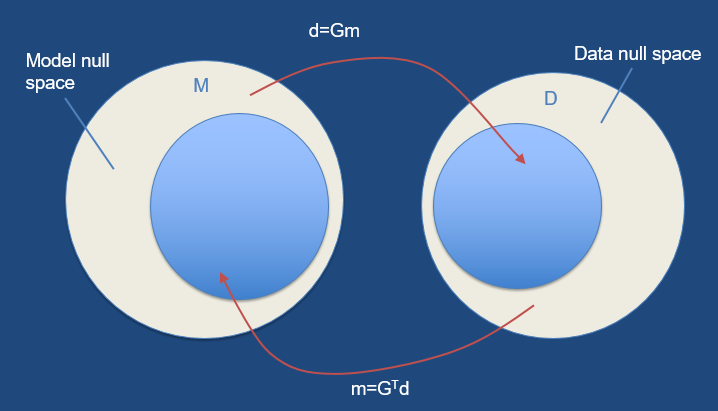
Now let us consider one inverse problem
$$d=Gm$$
where m ∈ M is some function (or vector) from a real Hilbert space M of the model parameters, and d ∈ D is an element from a real Hilbert space D of data sets, and G is a nonlinear operator.
This problem can be solved directly in the case of the linear operator G of a forward modeling. In the general case of a nonlinear operator G, the solution can only be found iteratively. There are many different approaches to the construction of the iteration process for functional minimization. One of the most widely used techniques for optimization is based on gradient-type methods.
Different Gradient based optimization algorithms for a linear/linearized inverse problem are discussed below:
Method of Steepest Descent:
This algorithm tries to find the nearest local minimum of a function assuming that the gradient of the function can be computed. In this method we start with a starting model, say, \(m_{o}\), and take a series of steps until the algorithm converges. At each iteration, we move along the direction in which the error changes most rapidly, which happens to be the direction of the gradient. So the method of steepest descent is also called the gradient descent method. Now, if the aim is to find the minimum of the cost function then the algorithm proceeds along a negative gradient direction calculated at each iteration. Gradient based methods also need a parameter defining the length of the ‘jump’ to be performed at each step. It can be taken as a constant or it may also be optimized in each iteration. If it is taken too small, the algorithm converges too slowly and if it is taken too large, the algorithm may diverge, in other words, if the step size is large, there is a possibility that the algorithm will overshoot the minimum point and become oscillatory. In order to avoid such a situation, the step size is calculated by computing the optimum step size at every iteration. This is done by computing the first order derivative with respect to the step size and equating to zero. But as the iteration goes on it becomes smaller and smaller and the process becomes very slow.
We can start by formulating the inverse problem as $$d=Gm$$
The linear least squares problem tries to minimize the error between the observed and the predicted data. So the error can be expressed as, $$e=(Gm - d)$$ In least squares problem we tries to minimize the L2 norm of this error, thus $$e^Te = (Gm - d)^T(Gm - d)$$ So, we can write the criterion of the linear least squares problem as $$min \ f(m) = min \ \left\Vert Gm-d \right\Vert _2^2$$ Now the objective function f (m) can be written as $$f (m) = (Gm − d)^T (Gm − d) = m^TG^TGm − 2(G^Td)^Tm + d^Td$$ If we take derivative of f(m) and then make equal to zero then, $$\frac{d}{dm^T}f(m) =0$$ The gradient is $$\nabla f(m) = 2G^TGm-2G^Td$$ Using the step length \(\alpha_k\) and including the constant 2 in it, we can write the gradient descent iteration as $$m^{(k+1)}=m^{(k)}-\alpha_k(G^TGm^{(k)}-G^Td)$$ let $$p^{(k)}=G^TGm^{(k)}-G^Td$$ We can also define the residual vector as $$r^{(k)}=d-Gm^{(k)}$$ and thus $$p^{(k)}=-G^Tr^{(k)}$$ Therefore, $$m^{(k+1)}=m^{(k)}-\alpha_kp^{(k)}$$ We can now compute \(f (m^{(k+1)})\) as
\begin{equation} \begin{split} f (m^{(k+1)}) & = (Gm^{(k+1)}-d)^T (Gm^{(k+1)}-d) \\ & = (G(m^{(k)}-\alpha_kp^{(k)})-d)^T (G(m^{(k)}-\alpha_kp^{(k)})-d) \\ & = (-r^{(k)}-\alpha_kGp^{(k)})^T (-r^{(k)}-\alpha_kGp^{(k)}) \\ & =r^{(k)^T }r^{(k)}+2\alpha_kp^{(k)^T}G^Tr^{(k)}+\alpha_k^2p^{(k)^T}G^TGp^{(k)}\\ \end{split} \end{equation} Since \(f(m^{(k)}) = r^{(k)^T}r^{(k)}\), we have \begin{equation} f (m^{(k+1)})-f(m^{(k)})=2\alpha_kp^{(k)^T}G^Tr^{(k)}+\alpha_k^2p^{(k)^T}G^TGp^{(k)} \end{equation} Since \(p^{(k)}=-G^Tr^{(k)}\) \begin{equation} \begin{split} f (m^{(k+1)})-f(m^{(k)}) &=-2\alpha_kp^{(k)^T}p^{(k)}+\alpha_k^2p^{(k)^T}G^TGp^{(k)}\\ & =p^{(k)^T}(-2\alpha_kI+\alpha_k^2G^TG)p^{(k)} \end{split} \end{equation} The decrease in the objective function value from iteration k to iteration k + 1 is thus $$f(m^{(k)})- f (m^{(k+1)})=p^{(k)^T}(2\alpha_kI-\alpha_k^2G^TG)p^{(k)}$$ Let \( \lambda_{max}(G^TG) \) be the largest eigenvalue of \(G^TG\) and also consider the matrix \(H=2\alpha_kI-\alpha_k^2G^TG\) . If $$2\alpha \ge \alpha_k^2 \lambda_{max}(G^TG)$$ then, H is positive definite and \(f (m^{(k+1)}) < f(m^{(k)})\). The associated condition on \(\alpha_k\) is thus $$\alpha_k\le \frac{2}{\lambda_{max}(G^TG)}$$However, if \(\alpha_k\) is larger than the critical value \(2/\lambda_{max}\) then H will not be positive definite, and depending on the value of \(p^{(k)}\), the objective function value might increase from iteration k to k+1. One simple approach to selecting \(\alpha_k\) is to pick a constant value \(\alpha_k=\omega\) such that $$\alpha_k=\omega< \frac{2}{\lambda_{max}(G^TG)}$$
This ensures that the objective function f is reduced at each iteration.
Another approach, in selecting \(\alpha_k\) the approach of exact line search is implemented, to find the value of \(\alpha_k\) that achieves the greatest possible decrease in the objective function. $$max \ g(\alpha) =f(m^{(k)})- f (m^{(k+1)})=2\alpha_kp^{(k)^T}p^{(k)}-\alpha_k^2p^{(k)^T}G^TGp^{(k)}$$ Differentiating with respect to \(\alpha\) and setting the derivative equal to zero. $$g'(\alpha)=0 $$ $$2p^{(k)^T}p^{(k)}-2\alpha_kp^{(k)^T}G^TGp^{(k)}=0 $$ $$\alpha_k=\frac{p^{(k)^T}p^{(k)}}{p^{(k)^T}G^TGp^{(k)}}$$ Since this includes expensive multiplication of \(G^TG\) $$\alpha_k=\frac{p^{(k)^T}p^{(k)}}{(Gp^{(k)})^T(Gp^{(k)})}$$
There is a drawback to steepest descent, which occurs when the ratio of the largest to the smallest eigenvalue (the condition number κ) is very large. Also this method becomes very slow while reaching towards the solution.
The algorithm for the steepest descent algorithm is provided below.
Governing eqn $$m^{(k+1)}=m^{(k)}-\alpha_kp^{(k)}$$ 1: Given m0;
2: Set k = 0;
3: while (Convergence criteria not satisfled) do
4: \(p^{(k)}=-G^Tr^{(k)}\)
5: if \(p^{(k)} = 0 \) then
6: Stop
7: end if
8: \(\alpha_k=\frac{p^{(k)^T}p^{(k)}}{(Gp^{(k)})^T(Gp^{(k)})}\)
9: \(m^{(k+1)}=m^{(k)}-\alpha_kp^{(k)}\)
10: k = k + 1 11: end while
Below Figure 4 shows the flowchart for steepest descent algorithm.

Figure 4: Flowchart for steepest descent algorithm.
In Figure 5 shows the contours of the constant cost function values. The arrows show the direction in which the steepest descent algorithm proceeds.

Figure 5: Convergence in steepest descent algorithm.

Figure 6: The plot of the misfit functional value as a function of model parameters m.
The intersection between the vertical plane P drawn through the direction of the steepest descent at point mn and the misfit functional surface is shown by a solid parabola type curve. The steepest descent step begins at a point φ (mn) and ends at a point φ (mn+1) at the minimum of this curve. The second parabola-type curve (on the left) is drawn for one of the subsequent iteration points. Repeating the steepest descent iteration, we move along the set of mutually orthogonal segments, as shown by the solid arrows in the space M of the model parameters.
Method of Conjugate Gradient:
Global Optimization:
Unlike local optimization methods, these methods attempt to i nd the global minimum of the misi t function. Most of the global optimization algorithms are stochastic in nature and use more global information about the misi t surface to update their current position. The convergence of these methods to the globally optimal solution is not guaranteed for all the algorithms. Only for some of the simulated annealing algorithms under certain conditions is convergence to the globally optimal solution statistically guaranteed. Also, with real observational data it is never possible to know whether the derived solution corresponds to the global minimum or not.