Null space

If the seismic velocity in the earth depends only on depth, the velocity can be constructed exactly from the measurement of the arrival time as a function of distance. 

Fig1: The traditional definition of the forward and inverse problems

Despite the mathematical elegance of the exact nonlinear inversion schemes, they are of limited applicability. There are a number of reasons for this.

• First, the exact inversion techniques are usually only applicable for idealistic situations that may not hold in practice.

• Second, the exact inversion techniques often are very unstable.

• Third reason is the most fundamental. In many inverse problems the model that one aims to determine is a continuous function of the space variables. This means that the model has infinitely many degrees of freedom. However, in a realistic experiment the amount of data that can be used for the determination of the model is usually finite. A simple count of variables shows that the data cannot carry sufficient information to determine the model uniquely.

The fact that in realistic experiments a finite amount of data is available to reconstruct a model with infinitely many degrees of freedom necessarily means that the inverse problem is not unique in the sense that there are many models that explain the data equally well. The model obtained from the inversion of the data is therefore not necessarily equal to the true model that one seeks. This implies that the view of inverse problems as shown in fig1 is too simplistic. For realistic problems, inversion really consists of two steps. 

Fig2: Inverse problem as a combination of 

an estimation problem and an appraisal problem.

Let the true model be denoted by m and the data by d. From the data d one reconstructs an estimated model \(m^{est}\), this is called the estimation problem (Fig2). Apart from estimating a model \(m^{est}\) that is consistent with the data, one also needs to investigate what relation the estimated model \(m^{est}\) bears to the true model m. 

In the appraisal problem one determines what properties of the true model are recovered by the estimated model and what errors are attached to it. Thus, $$inversion = estimation + appraisal$$In general there are two reasons why the estimated model differs from the true model. The first reason is the non-uniqueness of the inverse problem that causes several (usually infinitely many) models to fit the data. Technically, this model null-space exits due to inadequate sampling of the model space. The second reason is that real data are always contaminated with errors and the estimated model is therefore affected by these errors as well. 

Therefore model appraisal has two aspects, non-uniqueness and error propagation. 

Model estimation and model appraisal are fundamentally different for discrete models with a finite number of degrees of freedom and for continuous models with infinitely many degrees of freedom. Also, the problem of model appraisal is only well-solved for linear inverse problems. For this reason the inversion of discrete models and continuous models is treated  separately, and the case of linear inversion and nonlinear inversion is also treated independently.

Despite the mathematical elegance of the exact nonlinear inversion schemes, they are of limited applicability. There are a number of reasons for this. 

Null space

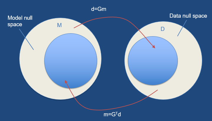
The vector d of the realisations can be related by a linear function to the vector of model parameters as:$$d=Gm \tag{1}$$where, G is an M x N matrix, and m and b are vectors of dimension N and M respectively. Equation (1) defines G as a linear mapping from an N-dimensional vector space to (generally) an M-dimensional one. But the map might be able to reach only a lesser-dimensional subspace of the full M-dimensional one. That subspace is called the range of G. The dimension of the range is called the rank of G. Sometimes there are nonzero vectors \(m_0\) that are mapped to zero by G, that is, \(Gm_0=0\). The space of such vectors (a subspace of the N-dimensional space that \(m_0\) lives in) is called the nullspace of G, and its dimension is called G’s nullity. The nullity can have any value from zero to N.

System (1) is usually either under- or over-determined, and a least squares solution is sought; unfortunately, we rarely get a unique and reliable solution because it is rank deficient. In fact, the so-called null space exists, constituted by vectors \(m_0\) being solution of the associated homogeneous system:$$Gm_0=0\tag{2}$$
Any linear combination of vectors \(m_0\) with a solution of (1) still satisfies system (1), and therefore the number of possible solutions is infinite in this case.

Singular value decomposition (SVD) allows to express matrix G by the following product:$$A = USV^T$$where: \(U^TU = I\), \(V^TV = VV^T = I\) , and I is the identity matrix. 

The elements \(s_{ij}\) of the diagonal matrix S are the singular values of G. The columns of the matrix V corresponding to null singular values constitute an orthonormal basis of the nullspace, whilst the columns of U corresponding to non-null singular values are an orthonormal base of the range.

Null space Example:

The vector of realizations d can be related by a linear function to the vector of model parameters m as z: $$d=Gm$$ Let us suppose that the inverse problem has two distinct solutions m1 and m2.

So, $$Gm1=d$$
and $$Gm2=d$$
Subtracting these two equations yields
$$G(m1-m2)=0$$
Since, the two solutions are by assumptions distinct, their difference $$m_0=m_1-m_2$$ is non-zero.

The converse is also true, any linear inverse problem that has null vectors then it has non-unique solution. If \(m_{par}\) (particular) is an non-null solution to \(Gm=d\), for instance minimum length solution, then \(m_{par}+\alpha m_0\), is also a solution any choice of \(\alpha\). 

Note that since \(\alpha m_0\) is a null vector for any non-zero \(\alpha\), null vectors are only distinct if they are linearly independent. 

If a given inverse problem has a q distinct null solutions, then most general solution  $$m_{gen}=m_{par}+\sum_{i=1}^{q} \alpha_i m_0$$

 

The data null space

Linear combinations of data that cannot be predicted by any possible model vector m. For example, no simple linear theory could predict different values for a repeated measurement, but real repeated measurements will usually differ due to measurement error. If there is a data null space, and if the data have a component in this null space, then it will be impossible to fit them exactly.

The model null space

A model null vector is any solution to the homogenous problem $$Gm_{0}=0$$This means we can add in an arbitrary constant times any model null vector and not affect the data misfit. So, the existence of a model null space implies non-uniqueness of any inverse solution.

Both a Model and a Data Null Space 

In the case of a data null space, we saw that the generalized inverse solution minimized the least squares mis-fit of data and model response. While in the case of a model null space, the generalized inverse solution minimized the length of the solution itself. If there are both model and data null spaces, then the generalized inverse simultaneously optimizes these goals.

Null space from SVD

Column vectors of U associated with 0 (or very near-zero) singular values are in the data null space. 

Column vectors of V associated with 0 singular values are in the model null space.

Minimum length solution never contains any null vectors. But if we use other solution simply(flatness/roughness), those solutions will contain null vectors.