A magnetometer is a device that measures magnetism - the direction, strength, or relative change of a magnetic field at a particular location.
Magnetic fields
Magnetic fields are vector quantities characterized by both
strength and direction. The strength of a magnetic field is measured in units
of tesla in the SI units, and in gauss in the cgs system of units. Measurements
of the Earth's magnetic field are given in units of nanotesla (nT), also
called a gamma. The Earth's magnetic field can vary from 20,000 to 80,000 nT
depending on geolocation, fluctuations in the Earth's magnetic field are of the
order of 100 nT, and magnetic field variations due to magnetic anomalies can be
in the picotesla (pT) range. Gaussmeters and Teslameters are magnetometers that
measure in units of gauss or tesla, respectively.
Types of Magnetometer
Depending on the types of measurement magnetometer are of two types:
- Vector magnetometers measure the vector components of a magnetic field.
- Total field magnetometers or scalar magnetometers measure the magnitude of the vector magnetic field.
Note: A magnetograph is a
magnetometer that continuously records data.
Magnetometers can also be classified as "AC" if
they measure fields that vary relatively rapidly in time (>100 Hz), and
"DC" if they measure fields that vary only slowly (quasi-static) or
are static. AC magnetometers find use in electromagnetic systems (such as
magnetotellurics), and DC magnetometers are used for detecting mineralisation
and corresponding geological structures.
Example of scalar and vector magnetometers include Caesium vapour and Fluxgate magnetometers, respectively.
Specification of Magnetometer
The performance and capabilities of magnetometers are described through their technical specifications. Major specifications include
|
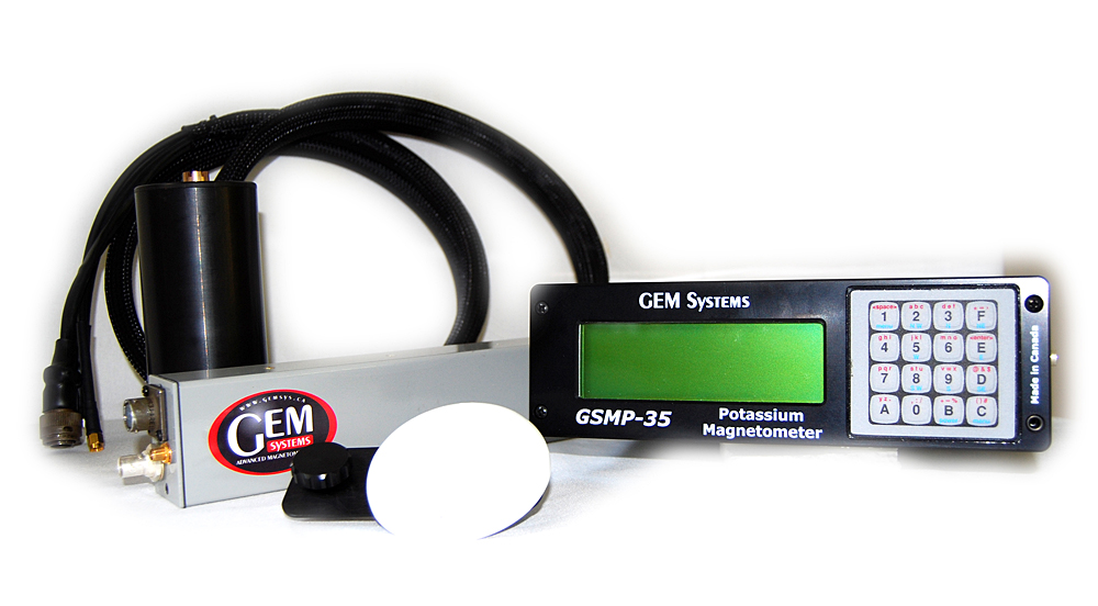
GSM19-T Technical Specifications Sensitivity: 0.15 nT @ 1 reading per sec i.e., 1Hz or 0.05 nT @ 1 reading every 4 sec Resolution: 0.01 nT Absolute Accuracy: +/- 0.2 nT @ 1 Hz Dynamic Range: 20,000 to 120,000 nT Gradient Tolerance: over 7000 nT/m Samples at: 60+, 5, 4, 3, 2, 1, 0.5 sec Operating Temperature: -40°C to +50°C Operating Modes: Manual- coordinates, time, date and reading stored automatically (GSM-19T: 3s, 19TW: 0.5s, 19TGW: 0.5s) Base Station- time, date and reading stored at 3(or 0.5) to 60 second intervals. Manufacturer: GEM Systems |
Scalar Magnetometers
1. Proton precession
magnetometer
Proton precession magnetometers (also known as proton
magnetometers, PPMs or simply mags) measure the resonance frequency of protons
(hydrogen nuclei), in the magnetic field to be measured, due to nuclear magnetic
resonance (NMR). Because the precession frequency depends only on atomic
constants and the strength of the ambient magnetic field, the accuracy of this
type of magnetometer can reach 1 ppm(parts-per-million).
A direct current flowing in a solenoid creates a strong
magnetic field around a hydrogen-rich fluid (Kerosene and Decane are popular, and even water can be used), causing some of the protons to align themselves with
that field. The current is then interrupted, and as protons realign themselves
with the ambient magnetic field, they precess at a frequency that is directly
proportional to the magnetic field. This produces a weak rotating magnetic
field that is picked up by a (sometimes separate) inductor, amplified
electronically, and fed to a digital frequency counter whose output is
typically scaled and displayed directly as field strength or output as digital
data.
PPMs work in field gradients up to 3,000 nT/m, which is
adequate for most mineral exploration work. For higher gradient tolerance, such
as mapping banded iron formations and detecting large ferrous objects,
Overhauser magnetometers can handle 10,000 nT/m, and caesium magnetometers can
handle 30,000 nT/m.
They are relatively inexpensive (< US$8,000) and were
once widely used in mineral exploration. Three manufacturers dominate the
market: GEM Systems, Geometrics and Scintrex. Popular models include G-856/857, Smartmag,
GSM-18, and GSM-19T.
For mineral exploration, they have been superseded by
Overhauser, caesium, and potassium instruments, all of which are fast-cycling,
and do not require the operator to pause between readings.
Overhauser effect
magnetometer
The Overhauser effect magnetometer or Overhauser magnetometer uses the same fundamental effect as the proton precession magnetometer to take measurements. By adding free radicals to the measurement fluid, the nuclear Overhauser effect can be exploited to significantly improve upon the proton precession magnetometer. Rather than aligning the protons using a solenoid, a low power radio-frequency field is used to align (polarise) the electron spin of the free radicals, which then couples to the protons via the Overhauser effect. This has two main advantages: driving the RF field takes a fraction of the energy (allowing lighter-weight batteries for portable units), and faster sampling as the electron-proton coupling can happen even as measurements are being taken. An Overhauser magnetometer produces readings with a 0.01 nT to 0.02 nT standard deviation while sampling once per second.
2. Optically Pumped Magnetometer
Optically pumped magnetometers (OPMs) are, in principle,
scalar type quantum sensors for magnetic fields based on the Zeeman effect.
That is the shift of energy levels due to the interaction of atoms with an
external magnetic field. Usually alkali vapors in paraffin-coated glass cells
are used as sensing element.
The principle of operation may be understood from the below examination, which shows three possible energy levels, A1, A2, and B for a hypothetical atom. Under normal conditions of pressure and temperature, the atoms occupy ground state levels A1 and A2. The energy difference between A1 and A2 is very small (approx. 10^-8 electron volts), representing a fine structure due to atomic electron spins that normally are not all aligned in the same direction. Even thermal energies (~ 10^-2 eV) are much larger than this, so that the atoms are as likely to be in level A1 as in A2.
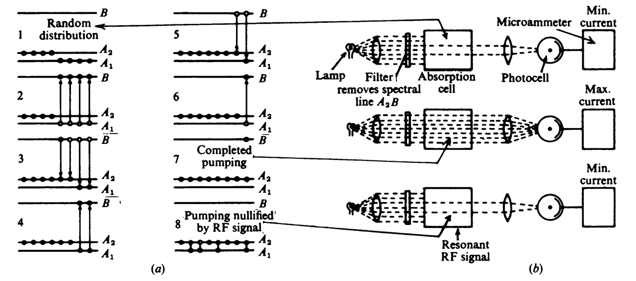
Level B represents a much higher energy and the transitions from A1 or A2 to B correspond to infrared or visible spectral lines. If we irradiate a sample with a beam from which spectral line A2B has been removed, atoms in level A1 can absorb energy and rise to B, but atoms in A2 will not be excited. When the excited atoms fall back to ground state, they may return to either level, but if they fall to A1, again they will be removed by photon excitation to B. The result is an accumulation of atoms in level A2.
The technique of overpopulating one energy level in this fashion is known as optical pumping. As the atoms are moved from level A1 to A2 by this selective process, less energy will be absorbed and the sample becomes increasingly transparent to the irradiating beam. When all atoms are in the A2 state, a photosensitive detector will register a maximum current. If now we apply an RF signal, having energy corresponding to the transition between A1 and A2, the pumping effect is nullified and the transparency drops to a minimum again. The proper frequency for this signal is given by v = E/h, where E is the energy difference between A1 and A2 and h is Planck's constant [6.62 x 10^-34 joule-seconds]. The energy difference between levels A1 and A2 is proportional to the strength of the ambient magnetic field.
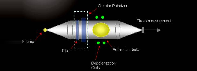
To make this device into a magnetometer, it is necessary to select atoms that have magnetic energy sublevels that are suitably spaced to give a measure of the weak magnetic field of the Earth. Elements that have been used for this purpose are alkali vapours which includes cesium, rubidium, sodium, potassiam and helium. The first three each have a single electron in the outer shell whose spin axis lies either parallel or antiparallel to an external magnetic field. These two orientations correspond to the energy levels A1 and A2 (actually the sublevels are more complicated than this, but the simplification illustrates the pumping action adequately), and there is a difference of one quantum of angular momentum between the parallel and antiparallel states. The irradiating beam is circularly polarized so that the photons in the light beam have a single spin axis. Atoms in sublevel A1 then can be pumped to B, gaining one quantum by absorption, whereas those in A2 already have the same momentum as B and cannot make the transition.
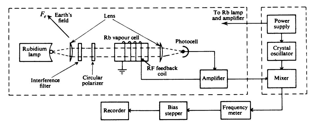
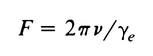
Above figure is a schematic diagram of the rubidium-vapor magnetometer. Light from the Rb lamp is circularly polarized to illuminate the Rb vapor cell, after which it is refocused on a photocell. The axis of this beam is inclined approximately 45° to the Earth's field, which causes the electrons to precess about the axis of the field at the Larmor frequency. At one point in the precession cycle the atoms will be most nearly parallel to the light-beam direction and one-half cycle later they will be more antiparallel. In the first position, more light is transmitted through the cell than in the second. Thus the precession frequency produces a variable light intensity that flickers at the Larmor frequency. If the photocell signal is amplified and fed back to a coil wound on the cell, the coil-amplifier system becomes an oscillator whose frequency v is given by
Caesium vapour magnetometer
The device broadly consists of a photon emitter, such as a laser, an absorption chamber containing caesium vapour mixed with a "buffer gas" through which the emitted photons pass, and a photon detector, arranged in that order. The buffer gas is usually helium or nitrogen and they are used to reduce collisions between the caesium vapour atoms.
The basic principle that allows the device to operate is the fact that a caesium atom can exist in any of nine energy levels, which can be informally thought of as the placement of electron atomic orbitals around the atomic nucleus. When a caesium atom within the chamber encounters a photon from the laser, it is excited to a higher energy state, emits a photon and falls to an indeterminate lower energy state. The caesium atom is "sensitive" to the photons from the laser in three of its nine energy states, and therefore, assuming a closed system, all the atoms eventually fall into a state in which all the photons from the laser pass through unhindered and are measured by the photon detector. The caesium vapour has become transparent. This process happens continuously to maintain as many of the electrons as possible in that state.
At this point, the sample (or population) is said to have been optically pumped and ready for measurement to take place. When an external field is applied it disrupts this state and causes atoms to move to different states which makes the vapour less transparent. The photo detector can measure this change and therefore measure the magnitude of the magnetic field.
In the most common type of caesium magnetometer, a very small AC magnetic field is applied to the cell. Since the difference in the energy levels of the electrons is determined by the external magnetic field, there is a frequency at which this small AC field makes the electrons change states. In this new state, the electrons once again can absorb a photon of light. This causes a signal on a photo detector that measures the light passing through the cell. The associated electronics use this fact to create a signal exactly at the frequency that corresponds to the external field.
Potassium vapour magnetometer
Potassium is the only optically pumped magnetometer that operates on a single, narrow electron spin resonance (ESR) in contrast to other alkali vapour magnetometers that use irregular, composite and wide spectral lines and helium with the inherently wide spectral line.
Advantages
The caesium and potassium magnetometers are typically used where a higher performance magnetometer than the proton magnetometer is needed.
The caesium and potassium magnetometer's faster measurement rate allows the sensor to be moved through the area more quickly for a given number of data points.
Caesium and potassium magnetometers are insensitive to rotation of the sensor while the measurement is being made.
The lower noise of caesium and potassium magnetometers allow those measurements to more accurately show the variations in the field with position.
Note: The dead zone is the angular region of magnetometer orientation in which the instrument produces poor or no measurements. All optically pumped, proton-free precession, and Overhauser magnetometers experience some dead zone effects.
Vector magnetometers
Vector magnetometers measure one or more components of the
magnetic field electronically. Using three orthogonal magnetometers, both
azimuth and dip (inclination) can be measured. By taking the square root of the
sum of the squares of the components the total magnetic field strength (also
called total magnetic intensity, TMI) can be calculated.
Magnetic gradiometers
The sensing elements of fluxgate, proton and optically pumped magnetometers can be used in pairs to measure either horizontal or vertical magnetic field gradients. Magnetic gradiometers are differential magnetometers in which the spacing between the sensors is fixed and small with respect to the distance of the causative body whose magnetic field gradient is to be measured.
Magnetic gradiometers are employed in surveys of shallow magnetic features as the gradient anomalies tend to resolve complex anomalies into their individual components, which can be used in the determination of the location, shape and depth of the causative bodies. The method has the further advantages that regional and temporal variations in the geomagnetic field are automatically removed.
Page in Establishing.......