A continuous-time (or analog) signal can be stored in a digital computer, in the form of equidistant discrete points or samples. The higher the sampling rate (or sampling frequency, \(f_S\)), the more accurate would be the stored information and the signal reconstruction from its samples. However, high sampling rate produces a large volume of data to be stored and makes necessary the use of a very fast analog-to-digital converter.
If the continuous signal observed between \(0 < t < T\) is digitized at \(\Delta t\) time intervals, discrete data will consist of \(N = (T/Δt) + 1\) discrete amplitude samples.
The maximum available frequency after digitization at regular \(\Delta t\) intervals is known as the Nyquist frequency \((f_N)\) and is determined only by the sampling interval. The Nyquist frequency is expressed as: $$f_N=\frac{1}{2\Delta t}$$
Nyquist-Shannon sampling theorem:
The minimum sampling frequency of a signal that it will not distort its underlying information, should be double the frequency of its highest frequency component.
Thus, if a function x(t) contains no frequencies higher than B hertz, it is completely determined by giving its ordinates at a series of points spaced 1/(2B) seconds apart. A sufficient sample-rate is therefore anything larger than 2B samples per second. Equivalently, for a given sample rate \(f_{s}\), perfect reconstruction is guaranteed possible for a bandlimit \(B<f_{s}/2\). \(f_s\)= 2B is called the Nyquist frequency.
If the signal g(t) had frequencies, for example, up to 140 Hz, then sampling at 4 ms, meaning that the maximum acquired frequency components of the signal is at f = 125 Hz, will cause a loss of the remaining 15 Hz of the original signal frequency band.
A continuous-time signal \(x(t)\) with frequencies no higher than fmax can be reconstructed exactly from its samples \(x[n] = x(nT_s)\), if the samples are taken a rate \(fs = 1/T_s\) that is greater than \(2f_{max}\). Note that the minimum sampling rate, \(2f_{max}\) , is called the Nyquist rate.
Oversampling
When we sample at a rate which is greater than the Nyquist rate, we say we are oversampling.
Undersampling and Aliasing
When we sample at a rate which is less than the Nyquist rate, we say we are undersampling and aliasing will yield misleading results.
Disruption of the spectrum because of the sparse sampling of a time signal is termed aliasing.
Aliasing occurs because: when digitized at \(\Delta t\) intervals, the analog \(f(t)\) signal is multiplied by a unit-amplitude comb function \(\delta (t-n\Delta t)\) in the time domain.
This multiplication produces a discrete time series \(f_r\), which consists of a series of amplitude values, mathematically expressed as $$f_r=f(n\Delta t)=f(t).\delta(t-n\Delta t)$$ $$=\sum_{-n}^{n}f_n(n\Delta t).\delta(t-n\Delta t$$
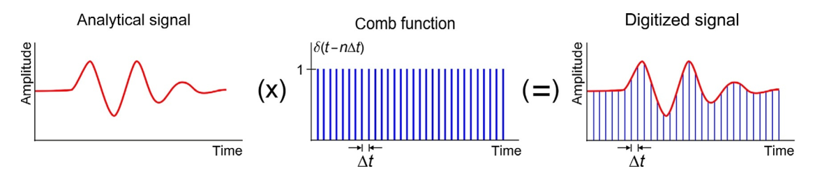
The digitized signal is multiplied by \(\delta (t-n\delta t)\), and multiplication in the time domain corresponds to their amplitude spectra being convolved in the frequency domain. The amplitude spectrum of a comb function is also a comb function sampled at \(\Delta t\) intervals. When the observed signal \(f(t)\) is digitized, this results in its amplitude spectrum \(F(\omega)\) being convolved with a comb function. As a consequence, \(F(\omega)\) becomes periodic along the frequency axis with a period of \(\Delta f\), and periodic recurrences of the discrete spectrum line up at \(\pm n/\Delta t\) intervals.
Because the widening in the frequency domain causes narrowing in the time domain, \(\Delta f\) becomes smaller as \(\Delta t\) gets larger. Therefore, high- and low frequency components of the periodic spectrum superimpose.
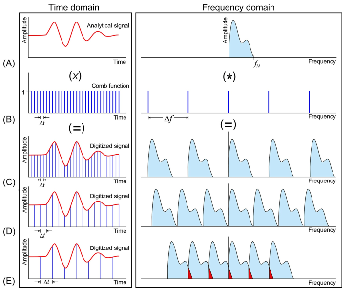
Degradation of the spectrum due to low frequency sampling using a sparse sampling interval presents practical issues. When \(f(t)\) is band limited, that is, when its maximum frequency is finite, the analog \(f(t)\) signal can be reconstructed from a digitized discrete signal \(f_r(t)\) without any information loss. In practice, however, such band-limited signals are rarely observed.
The sampling rate must be determined before recording during seismic acquisition. Yet, it is not practically possible to determine the appropriate sampling rate that is sufficiently small to prevent aliasing, because we do not know the highest frequency we record before shooting. Therefore, electronically designed low-pass and wide-band filter circuits, termed anti-aliasing filters, are designed. These are specific bandpass filters of wide passband and their higher frequency cutoff is generally 80% of the Nyquist frequency.
Mathematical procedure
A mathematically ideal way to interpolate the sequence involves the use of sinc functions. Each sample in the sequence is replaced by a sinc function, centered on the time axis at the original location of the sample, nT, with the amplitude of the sinc function scaled to the sample value, x[n]. Subsequently, the sinc functions are summed into a continuous function. A mathematically equivalent method is to convolve one sinc function with a series of Dirac delta pulses, weighted by the sample values. Neither method is numerically practical. Instead, some type of approximation of the sinc functions, finite in length, is used. The imperfections attributable to the approximation are known as interpolation error.
If \(f_S\) is the sampling frequency, then the critical frequency (or Nyquist limit) \(f_N\) is defined as equal to \(f_S/2\).
Any sinusoidal component of the signal of frequency \(f_m\) higher than \(f_N\) (e.g. \(f_m=f_N + \Delta f\)) is not only lost, but it is reintroduced in the sampled signal by folding at frequency \(f_N\) as an alias sinusoidal component of frequency \((f_m=f_N -\Delta f)\). This effect is known as aliasing.
When a sinusoidal signal of frequency f is sampled at frequencies greater than 2f, the sampling rates are adequate enough for the accurate reconstruction of the original sinusoidal signal, whereas if the sampling frequencies are less than 2f, subsampling occurs, and the collected points may be considered as belonging to signals of lower frequencies.
The alias frequencies due to subsampling can be calculated by the following equation: Alias frequency: \(f_a = | f - k f_S |\) where \(k=1,2,\ldots\)
For example: when \(f_S = 1.4f\), the alias frequency is \(f_a = | f - 1\times1.4f | = 0.4 f\), whereas, when \(fS / f = 0.8\), the alias frequency is \(f΄ = | f - 1x0.8f | = 0.2 f\)
The energy at frequencies higher than ωN folds back into the principal region (–ωN, ωN), known as the aliasing or edge folding phenomenon.