Cement Bond Log ~ Geo Markdown

The amplitude of an acoustic wave decreases as it propagates through a medium. This decrease is known as attenuation. It depends on several factors:

The wavelength of the wave and its type (longitudinal or transversal).
The texture of the rock (pore and grain size, type of grain contact, sorting), as well as the porosity, permeability and the specific surface of the rock pores.
The type of fluid in the pores and in particular its viscosity.
Rock fractures or fissures.

In cased wells the attenuation depends mainly on the quality of the cement around the casing. This can be indirectly measured by recording the sonic amplitude. This application is known as the Cement Bond Log (or CBL).

Different causes of attenuation

1. Loss of energy through heating

The vibration caused by the passage of a sonic wave causes energy loss in the form of heat. This loss of energy can have several interactions - Solid-to-solid friction, Solid-to-fluid friction or Fluid-to-fluid friction.

2. Redistribution of energy

2.1 Transfers along the media limits

A plane primary longitudinal wave moving in a solid M1, which presents a vertical boundary with a liquid M2 with the speed v2 and is less than that v1 in M1. The propagation of this wave causes undulation of the boundary moving towards the bottom through M1, which in turn generates a compressional wave in the medium M2. This secondary wave propagates in the direction P, forming an angle equal to the critical angle of incidence. with the original direction H,

The energy of the secondary wave comes from the primary wave and so a fraction of the original energy is transferred to the medium M2.

A transverse wave moving in the medium M1 also transfers part of its energy to M2 in the form of a compressional wave.

All this occurs in open hole along the borehole wall where the mud-formation boundary occurs and also in cased hole where the casing is not well cemented.

2.2 Transfers across media boundaries

When a wave crosses the boundary between two media M1 and M2 of different acoustic impedance we either have, depending on the angle of incidence, total reflection of the wave or part of the wave refracted into the medium M2 and part reflected back into M1. In the second case, there is attenuation of the wave.

This phenomenon is produced either at the boundary of formation and mud, or between layers of different lithologies or at fracture planes when the fractures are full of fluid or cemented.

In a cased hole it occurs at the boundaries of casing-cement-formation when the cement is good.

2.3 Dispersion

When the sonic wave encounters particles, whose dimensions are less than the wavelength, the sonic energy is dispersed in all directions, whatever is the shape of the reflection surface.

Different Attenuations happening in borehole

1. Open-hole

A) Attenuation in the mud

This is due the acoustic losses due to friction e.g., solid to fluid, and to dispersion losses at particles in suspension in the mud.

In a pure liquid this attenuation follows for one unique frequency:

$$\delta_{m}=e^{mx}$$

in which m is the attenuation factor in the liquid, proportional to the source of the frequency, and x is the distance over which the attenuation is measured.

For fresh water and at standard conditions of temperature and pressure, for a frequency of 20 kHz the attenuation factor is of the order of $3\times 10^{-5}$ db/ft.

It is higher for salt water and oil.
It decreases as the temperature and pressure increase.

For normal drilling muds which contain solid particles we have to add the effect of dispersion. It is estimated that the total dispersion is of the order of 0.03 db/ft for a frequency of 20 kHz.

In gas cut muds the attenuation caused by dispersion is very large, so making all sonic measurements impossible.

Note: Gas-cut mud: A drilling fluid (or mud) that has gas (air or natural gas) bubbles in it, resulting in a lower bulk, unpressurized density compared with a mud not cut by gas.

B) Attenuation by transmission

Attenuation by transmission of energy occurs at the mud-formation boundary for waves arriving at an angle of incidence less than critical.

C) Attenuation in the rock

(i) Frictional energy loss

In non-fractured rocks the attenuation of longitudinal and transverse waves is an exponential function of the form:

$$\delta_{F}=e^{al}$$

in which 'a' is the total attenuation factor due to different kinds of friction: solid to solid (a'), fluid to solid (a'') and fluid to fluid (a'''): a = a' + a'' + a'''

and l is the distance travelled by the wave. It is given by the equation:

$$l = L - (d_h - d_{tool})tgi_c$$

where L is the spacing, $d_h$ and $d_{tool}$, are the diameters of the hole and the tool, $i_c$ is the critical angle of incidence, which goes down as the speed in the formation increases.

When the rock is not porous, the factors a'' and a''' are zero.

When the rock is water saturated, a''' = 0.

In porous rocks, the attenuation factor a'' depends on the square of the frequency, whereas the factors a' and a''' are proportional to the frequency.

The factor a'' depends equally on porosity and permeability. It increases as the porosity and permeability increase.

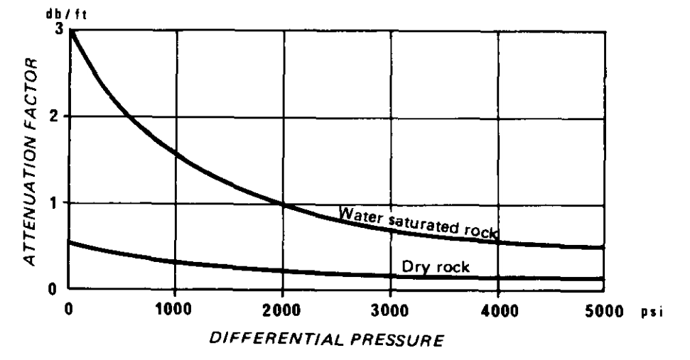
The attenuation factors a' and a'' decrease as the differential pressure $\Delta p$ (geostatic pressure - internal pressure of the interstitial fluids) increases.

Above figure , gives the relationship for dry rock - the energy losses are then due to solid to solid friction (a') and for water-saturated rock - the difference in attenuation (gap between the curves) is due to fluid to solid friction (a'').

When the rock contains hydrocarbons a greater attenuation of the longitudinal wave is observed in the case of gas than for oil (the factor a''' non zero).

From this we can deduce that the viscosity of the fluid has an effect on the attenuation factor a'''.

So, we can write that for a given tool considering all the different parameters acting on the attenuation:

$$a = F(f, v, \phi, k, S, \mu, \Delta p, \rho)$$

where,
           $f=$ frequency,
            $v=$ velocity of sound,
            $\phi=$ porosity,
            $k=$ permeability,
            $S=$ saturation,
            $\mu=$ viscosity of the fluids,
          $\Delta p=$ differential pressure and
          $\rho=$ density of the formation.

(ii) Loss of energy through dispersion and diffraction: this appears mainly in vuggy rocks.

D) Transmission across the boundaries of a medium

When a formation is made up of laminations of thin beds of different lithology at each boundary some or all of the energy will be reflected according to the angle of incidence. This angle is dependent on the apparent dip of the beds relative to the direction of the sonic waves. In the case of fractured rocks the same kind of effect occurs with the coefficient of transmission as a function of the dip angle of the fracture with regard to the propagation direction.

There is another effect due to transfer of energy along the borehole wall this part is already explained above.

2. Cased hole

The attenuation is affected by the casing, the quality of the cement and the mud.

If the casing is free and surrounded by mud, it can vibrate freely. In this case, the transfer factor of energy to the formation is low and the signal at the receiver is high. In some cases, even when the casing is free we can see the formation arrivals (on the VDL). This can happen if the distance between the casing and the formation is small (nearer than one or two wavelengths), or when the casing is pushed against one side of the well but free on the other. Transmission to the formation is helped by the use of directional transmitters and receivers of wide frequency response.

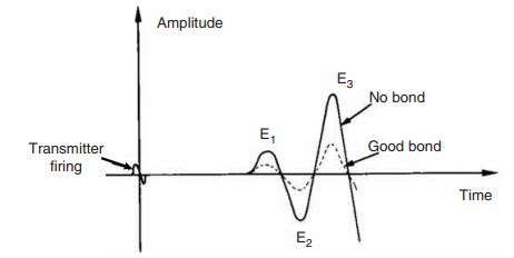
If the casing is inside a cement sheath that is sufficiently regular and thick (at least one inch) and the cement is well bonded to the formation the casing is no longer free to vibrate. The amplitude of the casing vibrations is much smaller than when the casing is free and the transfer factor to the formation is much higher. How much energy is transferred to the formation depends on the thickness of the cement and the casing. As energy is transferred into the formation the receiver signal is, of course, smaller.

Between the two extremes, well bonded casing and free pipe the amount of energy transferred and hence the receiver signal will vary.

Measurement

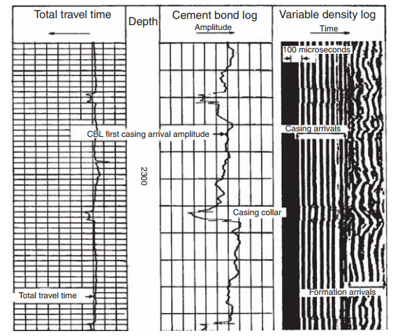
Cement Bond Log

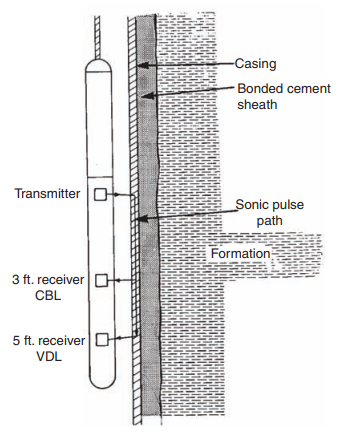
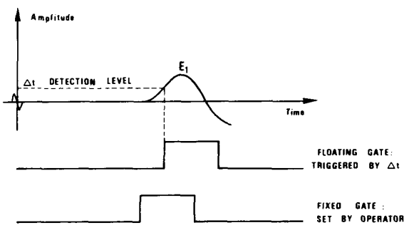
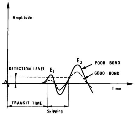
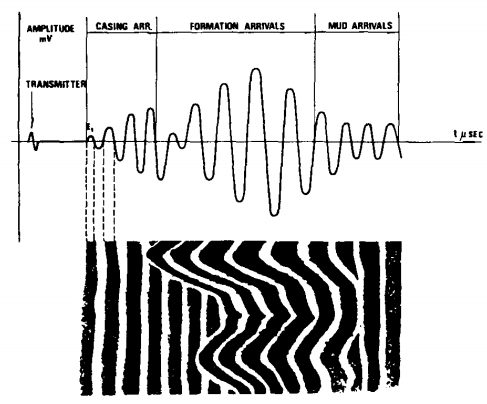
In the case of the Cement Bond Log (CBL), the general method is to measure the amplitude of the first arrival of the compressional wave at the receiver. These arrivals have a frequency between 20 and 25 kHz.

The amplitude of the first arrival is a function partly of the type of tool (particularly the tool spacing) and of the quality of the cementation: the nature of the cement and the percentage of the circumference of the tubing correctly bound to the formation.

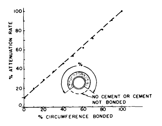
As we have seen the amplitude is a minimum, and hence the attenuation a maximum, when the tool is in a zone where the casing is held in a sufficiently thick annulus of cement (one inch at least). The amplitude is largest when the casing is free.

The amplitude is measured using an electronic gate (or window) that opens for a short time and measures the maximum value obtained during that time.

In the Schlumberger CBL (above fig.) there is a choice of two systems for opening the gate:

(a) Floating gate: the gate opens at the same point in the wave as the $\Delta t$ detection occurs and remains open for a time set by the operator, normally sufficient to cover the first half cycle. The maximum amplitude during the open time is taken as the received amplitude measurement.

(b) Fixed gate: the time at which the gate opens is chosen by the operator and the amplitude is measured as the maximum signal during the gate period. The fixed gate measurement is therefore independent of $\Delta t$.

Normally when $\Delta t$ is properly detected at El the two systems give the same result. If E1 is too small then $\Delta t$ detection will cycle skip to E3 (the case where the casing is very well cemented). The two systems then give: (a) fixed gate: El is still measured and is small; and (b) floating gate: El is measured and is usually large.

The measurement and recording of transit time at the same time as amplitude allows cycle skipping to be detected.

The interpretation of the CBL consists of the determination of the bond index which is defined as the ratio of the attenuation in the zones of interest to the maximum attenuation in a well cemented zone.

A bond index of 1 therefore, indicates a perfect bond of casing to cement to formation. Where the bond index is less than 1, this indicates a less perfect cementation of the casing. However, the bonding may still be sufficient to isolate zones from one another and so still be acceptable. Generally some lower limit is set on the bond index, above which the cementation is considered acceptable. The interpretation of the bond index is helped by the use of the Variable Density Log or VDL.

Attenuation can be calculated from the amplitude by using the charts, which also allows determination of the compressional strength of the cement. The transformation to attenuation from the amplitude measured in a CBL tool in millivolts depends mainly on the transmitter receiver spacing and smaller spacings (3 feet) always give better resolution than a large spacing.

Attenuation index

In its use in open hole Lebreton proposed a calculation of an index $I_c$ defined by the relation:

$$ I_c = (V_2 + V_3)/V_1 $$

where V1, V2 and V3 are the amplitude of the three first half-cycles of the compressional wave.

This index is also a function of the permeability as,

$$ I_c = \alpha log(k_v/\mu ) + \beta $$

where,

$k_v$= permeability measured along the axis of the core;

$\mu$ =viscosity of the wetting fluids in the rock;

$\alpha$ and $\beta$ are constants for a given tool and well.

It is not possible to record the whole wave using the CBL, except if we use the long-spacing sonic. In that case, we can record the entire signal.

Law of attenuation in open hole

By using experimental laboratory measurements Morlier and Sarda (1971) proposed the following equations for the attenuation of the longitudinal and transverse waves in a saturated porous rock:

$$S_p = 1.2 \times 10^{-3} \frac{S}{\phi} (2\frac{Mk}{\mu}f \rho_f)^{1/3}$$

$$S_s = 2.3 S_p$$

where;

S = specific surface (surface area of the pores per unit volume);

$\phi$ = porosity;

k = permeability;

$\rho_f$ = fluid density;

$\mu$ = fluid viscosity;

f = signal frequency.

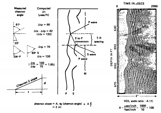
Variable density log (VDL)

A record is made of the signal transmitted along the logging cable during a 1000-$\mu$s period using a special camera. We can then either reproduce the trace by using an amplitude-time mode in which the wave train is shown as a wiggle trace otherwise translate it into a variable surface by darkening the area depending on the height of the positive half-waves of the sonic signal. This last method is known as the intensity modulated-time mode.

The different arrivals can be identified on the VDL as shown in below figure. Casing arrivals appear as regular bands whereas the formation arrivals are usually irregular. It is sometimes possible to distinguish amongst the arrivals between those linked with compressional waves and those with shear waves, by the fact that the latter arrive later and that they are at a sharper angle. They are often of higher energy (higher amplitude and therefore a darker trace).

In the case of the Schlumberger VDL the five foot receiver is used in order to improve the separation between waves.

Fig: Example of VDL chevron patterns on P and S waves.

VDL recording often has distinguishable chevron patterns. These are related to secondary arrivals caused by reflections and conversion of the primary waves at the boundaries of media with different acoustic characteristics, perhaps corresponding to: (a) bed boundaries; (b) fractures; (c) hole size variations; and (d) casing joints. Chevrons appear on longitudinal as well as transverse waves. Different appearance of this phenomenon is given in above figure.

The main applications of a study of chevron pattern are

(A) Fracture detection

Depending on the angle that the fracture planes make with the hole we have to consider three different cases:

(a) Fractures whose inclination is less than 35$^\circ$. The amplitude of the compression wave is hardly reduced. We can expect only a small amount of reflection. The VDL will have the following characteristics:

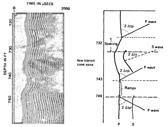
Strong amplitude of the compressional wave (E, or E2);
weak or no P-chevron pattern;
low amplitude of the shear waves; and
well defined S-chevron pattern.

(b) Fractures with an inclination between 35$^\circ$ and 85$^\circ$. The amplitude of the P-wave is reduced. The amplitude of the S-wave goes up and the VDL has the following characteristics:

low-amplitude P wave (E, and E2);
little or no S-chevron patterns; and
some P-chevron patterns.

(B) The calculation of $\Delta t$

This can be done if there are S-chevrons. In this case, $\Delta t$, is given by the gradient. We have

$$\Delta t_s= \frac{1}{2} d/t$$

The changes in $\Delta t_s$, are larger than those of $\Delta t_p$, which explains why the S-wave arrivals are not parallel to the P-wave arrivals. The difference in time between P- and S-wave arrivals can be approximated by the equation:

$T_s - T_p = (spacing) (\Delta t_s +\Delta t_p)$ from which we solve for $\Delta t_s$.

$$\Delta t_s = \Delta t_p +\frac{T_s - T_p}{spacing}$$

A real log example of CBL and VDL along with the total travel time is given below.